
ATCOR 2: Example Results
Basics | Features | Sensor Support | Methods | ATCOR-2 Results | ATCOR-3 Results
1. Haze Removal
The following mosaic shows part of a IRS-1C Liss-3 scene recorded 25 June 1998 (Craux, France). The left shows the original scene, the right is the processed surface reflectance scene employing ATCOR's haze removal algorithm in the hazy regions. Liss-3 bands 3, 2, 1 (NIR, Red, Green) are color coded RGB, respectively. The white areas are really haze regions of medium thickness in the original image, whilst the cloud-like appearance is caused by the JPEG image compression algorithm. However, the effect of clouds cannot be eliminated.

Another example shows part of an Ikonos scene of Dresden, 18 August 2002, �Space Imaging Europe 2002, demonstrating a successful haze removal. Ikonos bands 4, 2, 1 (NIR, Green, Blue) are color coded RGB, respectively.
 (80k)
(80k)The following figure shows surface reflectance spectra of decidous forest, coniferous forest, and bare soil calculated from a Landsat TM image. The two bare soil spectra were taken from clear and slightly hazy areas of the scene, depicting the correction capabilities of ATCOR haze removal.

2. Reflectance Image and Derived Automatic Surface Cover Classification
The following image shows a small part of the city of Dresden acquired by the
SPOT-3 sensor (22 April 1995).
The left section presents surface reflectance after atmospheric correction
(RGB=SPOT bands 3/2/1, NIR/Red/Green) and the right part shows the results of the automatic
spectral reflectance classification (program SPECL2: template reflectance spectra).
 (75k)
(75k)
Color coding of the classification map:
- dark to bright green : different vegetation covers
- blue : water
- brown: bare soil
- grey : asphalt, dark sand/soil
- white: bright sand/soil
- red : mixed vegetation/soil
- yellow: sun flower, rape (in bloom)
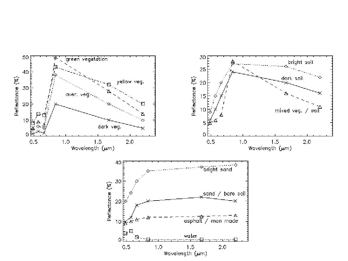
3. Template Reflectance Spectra of Program SPECL2
The following graph contains the template reflectance spectra employed by program SPECL2 to obtain the classification map. The symbols mark the Landsat TM / ETM+ center wavelengths. However, the program also works for sensors with fewer spectral bands, e.g. SPOT-1 to SPOT-4 or IRS-1C/-1D as demonstrated by the previous image.
4. Example of a Value Added Product: Net Radiation
The next image shows part of a Landsat-5 Scene of Munich (29 September 1991). The top part presents surface reflectance after atmospheric correction (RBG=TM bands 3/2/1) and the bottom presents the net radiation (Watts per square meter). It is calculated via the absorbed shortwave solar radiation plus downwelling atmospheric longwave radiation (requiring the air temperature and emissivity as input data) minus the emitted longwave surface radiation. The last components is computed from the thermal band of TM. Net radiation is an important quantity for hydrology, agriculture and climatology. It is the basis for determining heat fluxes (including ground heat flux, latent heat of evapotranspiration, and sensible heat flux).
 (192k)
Net radiation is high for surfaces with high absorption capabilities (low
albedo, integrated reflectance in the 0.4 - 2.5 um spectral region) and low surface
temperature, typical representatives are water bodies and dark vegetation
(coniferous forest).
Net radiation is low for surfaces of high albedo and/or high surface temperatures,
e.g. bright concrete surfaces, sand, bright bare soil and surfaces, warmed during the summer.
5. Water Vapor Map with Channels at 870, 940, 1010 nm
The next scene presents a mosaic of MOS-B imagery with the derived water vapor map. The MOS-B sensor was developed by DLR and operates onboard the Indian IRS-P3 satellite. MOS-B is mainly intended for the retrieval of water constituents for ocean and coastal zones. The instrument has a spatial resolution of 520 m. A scene consists of 384*384 pixels (200 km * 200 km). Data is recorded in 13 narrow spectral bands from 400 - 1010 nm with a spectral bandwidth of 10 nm. Although mainly intended for ocean applications, useful data products can also be generated for land applications.
The following example shows imagery recorded on 20 August 1996 (part of Northern Germany, RGB=868/615/484 nm, left part of mosaic). The right part of the mosaic presents the water vapor column derived over land. The water vapor values of the color ramp range from 0.3 to 1.9 g/cm2 for this scene. The water vapor is calculated with the APDA algorithm, see references and the ATCOR2 documentation .
6. Cirrus removal
Currently, no hyperspectral satellite sensor with the required 1.38 or 1.88 mciron band(s) and a sufficient
radiometric accuracy for cirrus removal is available.
Therefore, a high altitude (20 km) AVIRIS scene is substituted here to demonstrate that a cirrus removal
algorithm is available if this type of instrument is successfully launched. The method also works for multispectral
sensors, provided a narrow band around 1.38 micron exists, e.g., Sentinel-2.
The next figure presents an AVIRIS scene acquired on 6th April 1996 over Palmdale, CA and Bowie, MD (Courtesy of JPL).
The left part shows the original scene, the right part is the result after cirrus removal.
Thin and even very thick cirrus clouds are successfully removed.
The color coding is RGB = bands 858, 646, 547 nm.
 corr:
corr:

Example 2:
 corr:
corr:
